선형대수 기초 수식 LaTeX표현과 numpy 구현 with ChatGPT

논문에서 보이는 선형대수 식은 대부분 LaTeX 문법으로 작성된다. 나는 LaTeX 문법을 잘 모르지만 ChatGPT를 활용하여 간단한 선형대수식을 작성해 보았다.

Scalar : a single number

$ s \in \mathbb{R} $

Vector : an ordered list of numbers 

$ \mathbf{x} = \begin{bmatrix}1 \\ 2 \\ 3\end{bmatrix}, \mathbf{x} \in \mathbb{R}^3 $

Matrix : a two-dimensional array of numbers

$ \mathbf{A} = \begin{bmatrix}1 & 2 \\ 3 & 4 \\ 5 & 6\end{bmatrix}, \mathbf{A} \in \mathbb{R}^{3 \times 2} $

 

LaTeX 문법은 다음과 같다.

$ s \in \mathbb{R} $

$ \mathbf{x} = \begin{bmatrix}1 \\ 2 \\ 3\end{bmatrix}, \mathbf{x} \in \mathbb{R}^3 $

$ \mathbf{A} = \begin{bmatrix}1 & 2 \\ 3 & 4 \\ 5 & 6\end{bmatrix}, \mathbf{A} \in \mathbb{R}^{3 \times 2} $

 

$\mathbf{A}^T$ : Transpose of Matrix 

$ \mathbf{A}^T = \begin{bmatrix} 1 & 3 & 5 \\ 2 & 4 & 6 \end{bmatrix} ,  \mathbf{A}^T \in \mathbb{R}^{2 \times 3} $

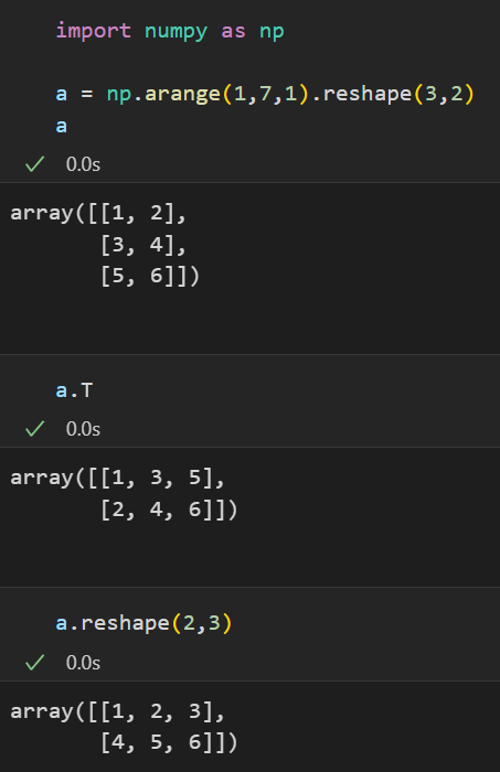
  Transpose는 Reshape와 다른 연산이다. 

 

 

Transpose 연산은 행렬을 대각선으로 뒤집는다. 딥러닝을 공부하다 보면 Attention 연산 등 자주 등장한다. 

$ \mathbf{A}_{ij} $ : i행 j열 위치의 원소(element)를 의미

$ \mathbf{A}_{12} = 2$

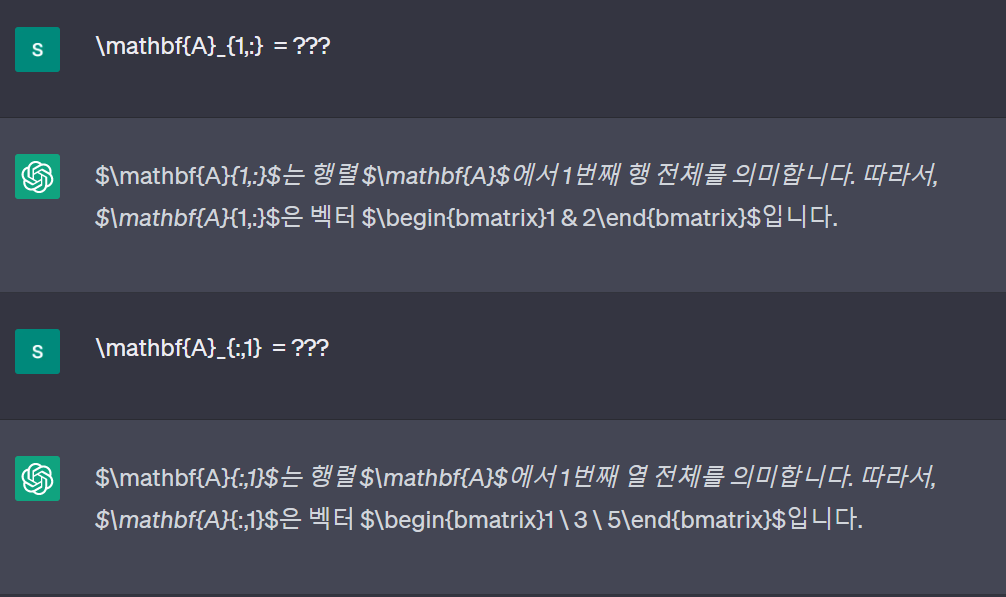
$ \mathbf{A}_{i,:} $ : i행의 모든 원소 (row vector)

$\mathbf{A}_{1,:} = \begin{bmatrix}1 & 2\end{bmatrix}$

$ \mathbf{A}_{:,j} $ : j열의 모든 원소 (column vector)

$\mathbf{A}_{:,1} = \begin{bmatrix}1 \\ 3 \\ 5\end{bmatrix}$

사용된 프롬프트 답변

다음은 스칼라, 벡터, 행렬 사이의 덧셈과 곱셈이다. 

1. 스칼라, 벡터 덧셈

$s + \mathbf{b} = \begin{bmatrix}s + b_1 \\ s + b_2 \\ \vdots \\ s + b_n \end{bmatrix}$

2. 스칼라, 행렬 덧셈

$s + \mathbf{A} = \begin{bmatrix}s + a_{11} & s + a_{12} & \cdots & s + a_{1m} \\ s + a_{21} & s + a_{22} & \cdots & s + a_{2m} \\ \vdots & \vdots & \ddots & \vdots \\ s + a_{n1} & s + a_{n2} & \cdots & s + a_{nm} \end{bmatrix}
$

3. 스칼라, 벡터 곱셈

$s \cdot \mathbf{b} = \begin{bmatrix}s \cdot b_1 \\ s \cdot b_2 \\ \vdots \\ s \cdot b_n \end{bmatrix}
$

4. 스칼라, 행렬 곱셈

$s \cdot \mathbf{A} = \begin{bmatrix}s \cdot a_{11} & s \cdot a_{12} & \cdots & s \cdot a_{1m} \\ s \cdot a_{21} & s \cdot a_{22} & \cdots & s \cdot a_{2m} \\ \vdots & \vdots & \ddots & \vdots \\ s \cdot a_{n1} & s \cdot a_{n2} & \cdots & s \cdot a_{nm} \end{bmatrix}
$ 

5. 벡터, 벡터 덧셈

$\mathbf{v} + \mathbf{w} = \begin{bmatrix} v_1 \\ v_2 \\ \vdots \\ v_n \end{bmatrix} + \begin{bmatrix} w_1 \\ w_2 \\ \vdots \\ w_n \end{bmatrix} = \begin{bmatrix} v_1 + w_1 \\ v_2 + w_2 \\ \vdots \\ v_n + w_n \end{bmatrix}
$

6. 행렬, 행렬 덧셈

$\mathbf{A} + \mathbf{B} = \begin{bmatrix} a_{11} & a_{12} & \cdots & a_{1n} \\ a_{21} & a_{22} & \cdots & a_{2n} \\ \vdots & \vdots & \ddots & \vdots \\ a_{m1} & a_{m2} & \cdots & a_{mn} \end{bmatrix} + \begin{bmatrix} b_{11} & b_{12} & \cdots & b_{1n} \\ b_{21} & b_{22} & \cdots & b_{2n} \\ \vdots & \vdots & \ddots & \vdots \\ b_{m1} & b_{m2} & \cdots & b_{mn} \end{bmatrix} = \begin{bmatrix} a_{11} + b_{11} & a_{12} + b_{12} & \cdots & a_{1n} + b_{1n} \\ a_{21} + b_{21} & a_{22} + b_{22} & \cdots & a_{2n} + b_{2n} \\ \vdots & \vdots & \ddots & \vdots \\ a_{m1} + b_{m1} & a_{m2} + b_{m2} & \cdots & a_{mn} + b_{mn} \end{bmatrix}
$

7. 행렬곱

$\mathbf{A} \mathbf{B} = \begin{bmatrix} a_{11} & a_{12} & \cdots & a_{1n} \\ a_{21} & a_{22} & \cdots & a_{2n} \\ \vdots & \vdots & \ddots & \vdots \\ a_{m1} & a_{m2} & \cdots & a_{mn} \end{bmatrix} \begin{bmatrix} b_{11} & b_{12} & \cdots & b_{1p} \\ b_{21} & b_{22} & \cdots & b_{2p} \\ \vdots & \vdots & \ddots & \vdots \\ b_{n1} & b_{n2} & \cdots & b_{np} \end{bmatrix} = \begin{bmatrix} c_{11} & c_{12} & \cdots & c_{1p} \\ c_{21} & c_{22} & \cdots & c_{2p} \\ \vdots & \vdots & \ddots & \vdots \\ c_{m1} & c_{m2} & \cdots & c_{mp} \end{bmatrix}$

8. 행렬, 열백터 곱셈

$\mathbf{A} \mathbf{v} = \begin{bmatrix} a_{11} & a_{12} & \cdots & a_{1n} \\ a_{21} & a_{22} & \cdots & a_{2n} \\ \vdots & \vdots & \ddots & \vdots \\ a_{m1} & a_{m2} & \cdots & a_{mn} \end{bmatrix} \begin{bmatrix} v_1 \\ v_2 \\ \vdots \\ v_n \end{bmatrix} = \begin{bmatrix} \sum_{i=1}^{n} a_{1i} v_i \\ \sum_{i=1}^{n} a_{2i} v_i \\ \vdots \\ \sum_{i=1}^{n} a_{mi} v_i \end{bmatrix}
$

9. 행백터, 행렬 곱셈

$\mathbf{v} \mathbf{A} = \begin{bmatrix} v_1 & v_2 & \cdots & v_n \end{bmatrix} \begin{bmatrix} a_{11} & a_{12} & \cdots & a_{1n} \\ a_{21} & a_{22} & \cdots & a_{2n} \\ \vdots & \vdots & \ddots & \vdots \\ a_{n1} & a_{n2} & \cdots & a_{nn} \end{bmatrix} = \begin{bmatrix} v_1 a_{11} + v_2 a_{21} + \cdots + v_n a_{n1} & v_1 a_{12} + v_2 a_{22} + \cdots + v_n a_{n2} & \cdots & v_1 a_{1n} + v_2 a_{2n} + \cdots + v_n a_{nn} \end{bmatrix}
$

8. 행렬, 열백터 덧셈

$\mathbf{A} + \mathbf{v} = \begin{bmatrix} a_{11} & a_{12} & \cdots & a_{1n} \\ a_{21} & a_{22} & \cdots & a_{2n} \\ \vdots & \vdots & \ddots & \vdots \\ a_{m1} & a_{m2} & \cdots & a_{mn} \end{bmatrix} + \begin{bmatrix} v_1 \\ v_2 \\ \vdots \\ v_n \end{bmatrix} = \begin{bmatrix} a_{11} + v_1 & a_{12} + v_2 & \cdots & a_{1n} + v_n \\ a_{21} + v_1 & a_{22} + v_2 & \cdots & a_{2n} + v_n \\ \vdots & \vdots & \ddots & \vdots \\ a_{m1} + v_1 & a_{m2} + v_2 & \cdots & a_{mn} + v_n \end{bmatrix}
$

9. 행백터, 행렬 덧셈

$\mathbf{v} + \mathbf{A} = [v_1, v_2, \ldots, v_n] + \begin{bmatrix} a_{11} & a_{12} & \cdots & a_{1n} \\ a_{21} & a_{22} & \cdots & a_{2n} \\ \vdots & \vdots & \ddots & \vdots \\ a_{m1} & a_{m2} & \cdots & a_{mn} \end{bmatrix} = \begin{bmatrix} v_1 + a_{11} & v_2 + a_{12} & \cdots & v_n + a_{1n} \\ v_1 + a_{21} & v_2 + a_{22} & \cdots & v_n + a_{2n} \\ \vdots & \vdots & \ddots & \vdots \\ v_1 + a_{m1} & v_2 + a_{m2} & \cdots & v_n + a_{mn} \end{bmatrix}
$

위 식에서 곱셈 연산은 브로드캐스팅이 아닌 내적 연산으로 행렬이나 벡터의 차원이 변경될 수 있다.

아래는 numpy를 사용한 브로드캐스팅의 구현 예시이다. 연산에 벡터, 행렬의 순서는 상관이 없고 row_vector와 matrix를 곱할 때, 넘파이 내부에서 row_vector를 repeat하여 곱했음을 알 수 있다. 단, 행벡터는 행렬의 열, 열벡터는 행렬의 행과 같은 차원이어야 한다.

# 행백터 생성

row_vector = np.array([1, 2, 3])

row_vector_repeat = np.repeat([row_vector],4,axis=0)

# 열벡터 생성

column_vector = np.array([[1],

                          [2],

                          [3],

                          [4]])

# 행렬 생성

matrix = np.array([[1, 2, 3],

                   [4, 5, 6],

                   [7, 8, 9],

                   [10, 11, 12]])

print('row vector(3,) * matrix(4,3) \n',row_vector*matrix,end='\n\n')

print('matrix(4,3) * row vector(3,) \n',matrix*row_vector,end='\n\n')

print('row vector(4,3) * matrix(4,3) \n',row_vector_repeat*matrix,end='\n\n')

print('column vector(4,1) * matrix(4,3) \n',column_vector*matrix,end='\n\n')

print('matrix(4,3) * column vector(4,1) \n',matrix*column_vector,end='\n\n')

결과 :

row vector(3,) * matrix(4,3) 
 [[ 1  4  9]
 [ 4 10 18]
 [ 7 16 27]
 [10 22 36]]

matrix(4,3) * row vector(3,) 
 [[ 1  4  9]
 [ 4 10 18]
 [ 7 16 27]
 [10 22 36]]

row vector(4,3) * matrix(4,3) 
 [[ 1  4  9]
 [ 4 10 18]
 [ 7 16 27]
 [10 22 36]]

column vector(4,1) * matrix(4,3) 
 [[ 1  2  3]
 [ 8 10 12]
 [21 24 27]
 [40 44 48]]

matrix(4,3) * column vector(4,1) 
 [[ 1  2  3]
 [ 8 10 12]
 [21 24 27]
 [40 44 48]]

 

행벡터의 요소를 하나 추가했을 때 에러

ValueError: operands could not be broadcast together with shapes (4,) (4,3)

수식으로 표현된 내적(dot)연산의 구현은 다음과 같다.

# 행벡터 생성

row_vector = np.array([1, 2, 3])

# 열벡터 생성

column_vector = np.array([[1],

                          [2],

                          [3]])

# 행렬 생성

matrix = np.array([[1, 2, 3],

                   [4, 5, 6],

                   [7, 8, 9]])

# 행벡터와 행렬 곱셈

row_matrix_product = np.dot(row_vector, matrix)

print("행벡터 * 행렬 결과:")

print(row_matrix_product)

print()

# 행렬과 열벡터 곱셈

column_matrix_product = np.dot(matrix, column_vector)

print("\n행렬 * 열벡터 결과:")

print(column_matrix_product)

결과:

행벡터 * 행렬 결과:
[30 36 42]


행렬 * 열벡터 결과:
[[14]
 [32]
 [50]]

행벡터의 요소를 하나 추가했을 때 에러

ValueError: shapes (4,) and (3,3) not aligned: 4 (dim 0) != 3 (dim 0)